This is the second post about the Gurobi solver. We will explore a functionality called lazy constraints: instead of providing all the constraints to the solver at the beginning, we will start solving a relaxed version of the problem. Every time we find a temporary solution, we incrementally add the constraints violated by that solution. Thanks to the dual simplex method, adding constraints can be done efficiently by Gurobi. In this way, we avoid adding useless constraints, speeding up the final solution.
I refer again to the opt4ds repository for more examples and interesting instances.
The source code for the solution of the main example can be found here: tsp.py
The Traveling Salesman Problem
The Traveling Salesman Problem (or TSP) is a famous optimization problem, with unclear origin. We are given a set of cities and the distances between each pair. The goal is to find the shortest path visitin all the cities only once, and then going back to the start.
The TSP is known to be NP-hard. Many benchmark instances can be found in the TSPLIB project page.
Relaxed Formulation
We want to formulate the TSP as an ILP problem. A common and intuitive choice is to model it as a weighted graph problem. The $n$ cities, numbered from $0$ to $n-1$, are the vertices of a graph. The edge $(i,j)$ has weight corresponding to the distance between the $i$-th and the $j$-th city. Our solution is the minimal cost path visiting all the cities only once, and then going back to the start.
This formulation translates into ILP using the adjacency matrix: we define an $n\times n$ matrix $M$ of binary variables, such that $M_{ij} = 1$ if and only if the optimal path includes the edge $(i,j)$ (equivalently, if the $i$-th and $j$-th cities are directly connected in the optimal path). The objective to minimize is the lenght of the total path, which can be directly computed from the adjacency matrix as
where $l(i,j)$ is the weight of the edge $(i,j)$ (the distance between $i$ and $j$ by definition). The tricky part here are the constraints. First of all, the orientation of our path is irrelevant; hence, we want $M_{ij} = M_{ji}$ for each $i,j$. We call these symmetry constraints. Looking at the path, we have the so called degree-2 constraints: each vertex must have one entering and one exiting edge, or simply two active edges, since we do not have any orientation. Thanks to symmetry, it’s enough to impose for each $i$
\[\sum_j M_{ij} = 1.\]At a first glance, these constraints may seem enough to obtain a valid solution. However, we will see that this is not the case. Let’s sample $n=10$ random points and compute the adjacency matrix:
1
2
3
4
5
6
7
8
9
10
11
12
13
14
15
import math
import random
import gurobipy as gp
from gurobipy import GRB

random.seed(42)

# Number of points
n = 10
points = [(random.randint(0, 100), random.randint(0, 100)) for i in range(n)]

# Adjacency matrix
dist = {(i, j):
        math.sqrt(sum((points[i][k]-points[j][k])**2 for k in range(2)))
        for i in range(n) for j in range(i)}
Then define and solve our model:
1
2
3
4
5
6
7
8
9
10
11
12
13
model.optimize()

m = gp.Model()

# Variables
vars = m.addVars(dist.keys(), obj=dist, vtype=GRB.BINARY, name='e')

# Symmetry constraints
for i, j in vars.keys():
    vars[j, i] = vars[i, j]

# Degree-2 constraints
m.addConstrs(vars.sum(i, '*') == 2 for i in range(n))
However, if we plot the solution (the function plottour(model, points), adapted from here, can be found in the source file), we get something like this:
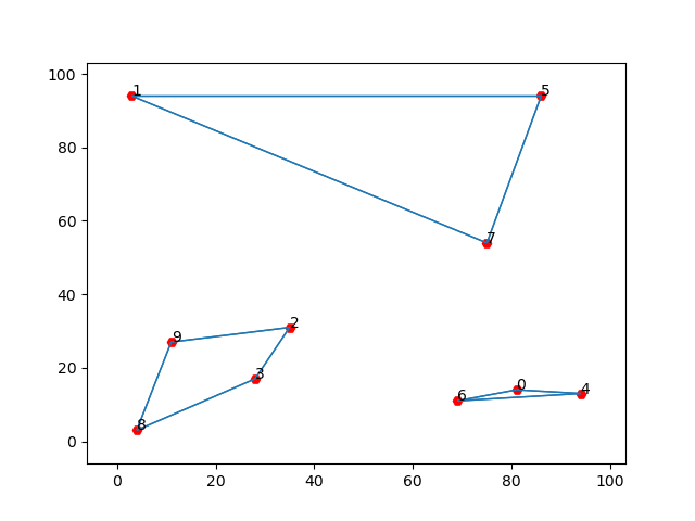
Subtour Elimination
Our solution contains three subtours, i.e. three paths visiting some of the points and then going back to the origin. We see that these subtours does not violate our degree-2 constraints: each city has only two active edge. This means that we have to add more constraints to obtain a proper solution. One way to do that is to check all the possible subtours and impose constraints to avoid them. This approach is known as the Dantzig-Fulkerson-Johnson (DFJ) formulation. Let’s move one step at a time. First of all, notice that our solution does not admit 2-subtours, i.e. subtours made by two cities. This is because for the symmetry constraints there is only one edge going from $i$ to $j$, and the degree-2 constraints impose that both $i$ and $j$ have two active edges. Let’s then move to the 3-subtours. If we have three cities, say $i$, $j$ and $k$, and we want to avoid a subtour connecting only these three, it’s enough to ask that the number of active edges containing only $i,j$ and $k$(due to symmetry again we only have $(i,j)$, $(j,k)$ and $(i,k)$) is less than $3$. This is a very simple condition. On the other hand, we need to impose this constraint for each triplet $(i,j,k)$ in a set of $n$ elements, which results in $\binom{n}{3}$ constraints. Similarly, to avoid 4-subtours we need that for any tuple $(i,j,k,l)$ the number of active edges containing only vertices in the tuple is less than $4$; this results in $\binom{n}{4}$ new constraints, and so on. We need to impose these constraints up to subsets of size $n-1$, since we are fine with a subtour of size $n$ (the actual solution). This means that the number of constraints we want to impose grows like the subsets of a set of $n$ elements, i.e. $\mathcal{O}(2^n)$, clearly too much for our problem.
Lazy Constraints
However, we notice that our prevoius solution has only three subtours, which means that it’s violating only three subtour constraints. Instead of adding all the $2^n$ constraints, which would not be feasible, we can try to iteratively add only the constraints that are violated by our solution, to break the subtours. In the previous example we want to impose 3-subtour constraints on the sets $(1,5,7)$ and $(0, 4, 6)$ and a 4-subtour constraint on the set $(2,3,8,9)$. Thanks to duality, adding constraints is quite efficient in practice, since we do not have to start solving the problem again from scratch, but we can partly exploit the prevoiusly found solution. In this way, we move from the current solution to a new one, which avoids these subtours but may create new ones. Iterating this process we add only the most important constraints, ignoring those that would not be violated by any possible optimal solution. At some point, hopefully way before $2^n$ iterations, we will get a valid solution with no subtours.
Let’s see how to implement this approach in Gurobi. First of all, we need to define a special function, called callback function, which takes two parameters as input: our model, and a status, which tells the function in which fase of the solving process is invoked.
1
2
3
4
5
6
7
8
9
10
11
12
13
14
from itertools import combinations

...

def subtourelim(model, status):
    if status == GRB.Callback.MIPSOL:
        n = model._ncities
        vals = model.cbGetSolution(model._vars)
        tour = subtour(vals, n) # Shortest cycle
        if len(tour) < n:
            # Subtour elimination
            model.cbLazy(
                gp.quicksum(model._vars[i, j] for i, j in combinations(tour, 2)) <= len(tour)-1
            )
subtour(vals, n) is an helper function that given the active edges in our model returns the shortest cycle tour. If its length is less then n then it’s a subtour, and we add a constraint to avoid it. Otherwise we are done. This callback function is automatically called by the solver; we only have to enable the LazyConstraints options:
1
2
3
4
5
6
7
8
9
10
11
12
13
m._ncities = n
m._vars = vars
m.Params.LazyConstraints = 1
m.optimize(subtourelim)

vals = m.getAttr('X', vars)
tour = subtour(vals, n)
assert len(tour) == n

plottour(m, points)

print('Optimal tour: %s' % str(tour))
print('Optimal cost: %g' % m.ObjVal)
Constraints analysis
This method is quite effective in practice: on my (old) laptop I can solve in about one minute instances with 200 random points. However, at this point one may ask how many constraints do we actually need, and more specifically how fast does this number grow with respect to $n$. To answer, we may simply check how many times our subtourelim function reports the condition len(tour) < n. For each $n$ from $5$ to $100$, I generated 10 random TSP instances and recorded the average number of constraints generated. The result is plotted against $n$ in the graph, compared with the function $y=x$ (source code here):
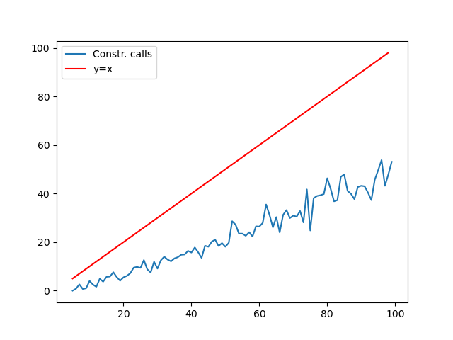
This confirms our intuition that only a small part of the $2^n$ total constraints are actually needed.